Decision Trees

Introduction

Decision trees form the foundations of powerful algorithms such as random forests and gradient boosting trees. They consist of a series of True or False questions asked about our independent variables to arrive at the target variable. In this article, we will take an illustrative tour of how the CART algorithm arrives at its final decision. We will use a classification problem involving the quality of wine(yes, wine!).

Cultivating a Decision Tree

We’ll use a the Red wine quality dataset from kaggle. Our task is to predict the quality of red wine based on a set of 9 independent variables. Let’s import the necessary libraries and our dataset.

import pandas as pd
import numpy as np
import matplotlib.pyplot as plt
%matplotlib inline

from sklearn.tree import DecisionTreeClassifier
from sklearn.tree import export_graphviz #plot tree

df = pd.read_csv('winequality-red.csv')

A quick glance at the data reveals that, our dependent variables contain classes that range from 3 - 8.

Let’s make it more readable by converting it to range from A - F: A mapping to 3, B => 4 in that order.

mappings_for_quality = {
    3:"A",
    4:"B",
    5:"C",
    6:"D",
    7:"E",
    8:"F"
}

df['quality'].replace(mappings_for_quality,inplace=True)

With all this in place, we can now train our decision tree on the data. For the sake of simplicity, we will limit our tree depth to 2.The depth illustrates how many levels of split we want. This is specified via the max_depth argument.

tree_classifier = DecisionTreeClassifier(max_depth=2)
df_x = df.copy()
X = df_x.drop('quality',axis=1)
y = df['quality']

tree_classifier.fit(X,y)

Visualizing the tree

We have successfully built a decision tree. We will now explore how our tree arrives at its decision. To do this, we use a function in the tree module of sklearn called Export_graphviz.

import os
from PIL import Image

path = '.'

from IPython.display import Image

from sklearn.tree import export_graphviz
from matplotlib.pyplot import imshow

def image_path(fig):
    return os.path.join(path,fig)

export_graphviz(
    tree_classifier,
    out_file=image_path("wine.dot"),
    feature_names=list(df_x.drop('quality',axis=1)),
    class_names=['C', 'D', 'E', 'B', 'F', 'A'],
    rounded=True,
    filled=True
)

!dot -Tpng wine.dot -o wine.png

Image(filename='wine.png')

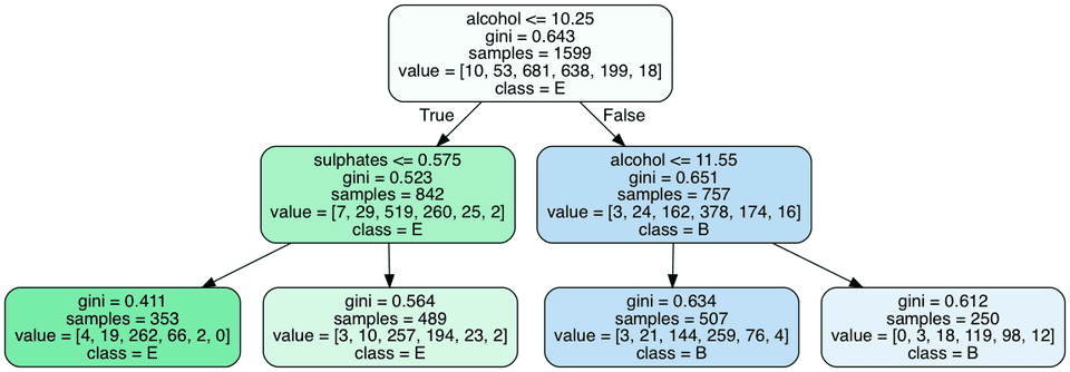
The code above plots a graph of the various decisions that occur at each node. Let’s examine the graph generated.

The figure above shows the steps our algorithm goes through to predict the class of wine. The first variable at the top is called the root node(depth=0). At each node, we have a feature, gini, samples, value and class. Let’s take time to explain what each of these terms mean:
feature - this is a feature the algorithm splits on. We’ll explore how this is done in a bit. Our features include fixed acidity,volatile acidity,citric acid,residual sugar,chlorides,free sulfur dioxide,total sulfur dioxide,density,pH,sulphates and alcohol.
gini - this is the value for the gini impurity. It represents the purity of a node. It is the cost function we for determining how good our splits are. A gini coefficient of 0 represents the pure node. Other cost functions include Chi-square,information gain and using the reduction in variance. The gini coefficient is calculated as\

$$ G = \sum_{i=1}^C p(i) * (1 - p(i)) $$

For our root node, G is calculated as

G = 1 - ( (10/1599)**2 + (53/1599)**2 + (681/1599)**2 + (638/1599)**2 + (199/1599)**2+ (18/1599)**2)

samples - This is the number of training instances in the node. From the image, the sample value at the root node is the entire dataset(1599). Also the sum of the sample values of the children node should be equal to that of the parent node. Eg. 842 + 757 = 1599.
value - How many training instances of each class is in that node. This values should sum up the samples value of that node.
class - predicted class of that node.

The decision making Process

For a classification problem like the wine problem, the algorithm splits on all possible features. It then searches for a pair of (feature,threshold) split that gives the purest(lowest gini coefficient) children nodes. In our case, the best split was on (alcohol, 10.45). The children node also undergo the same split process until we arrive at a pure node or a near pure node. When a new feature is fed to the decision tree, it traces the path it created and arrives at a leaf node. The target class in the leaf node becomes our predicted class.

Conclusion

In this post, we explored how the decision tree algorithm works. We trained on a wine quality dataset and explored the various components of our decision tree. While the training accuracy of decision tree is poor, it can help us understand our data better. We can identify the most predictive features and reason through how our models arrives at a final prediction. With decision trees out of the way, we can now focus on other tree based algorithms. In our next post, we will take a deep dive into random forests. We will explore the theory behind it as well as how to apply random forests in practical situations.